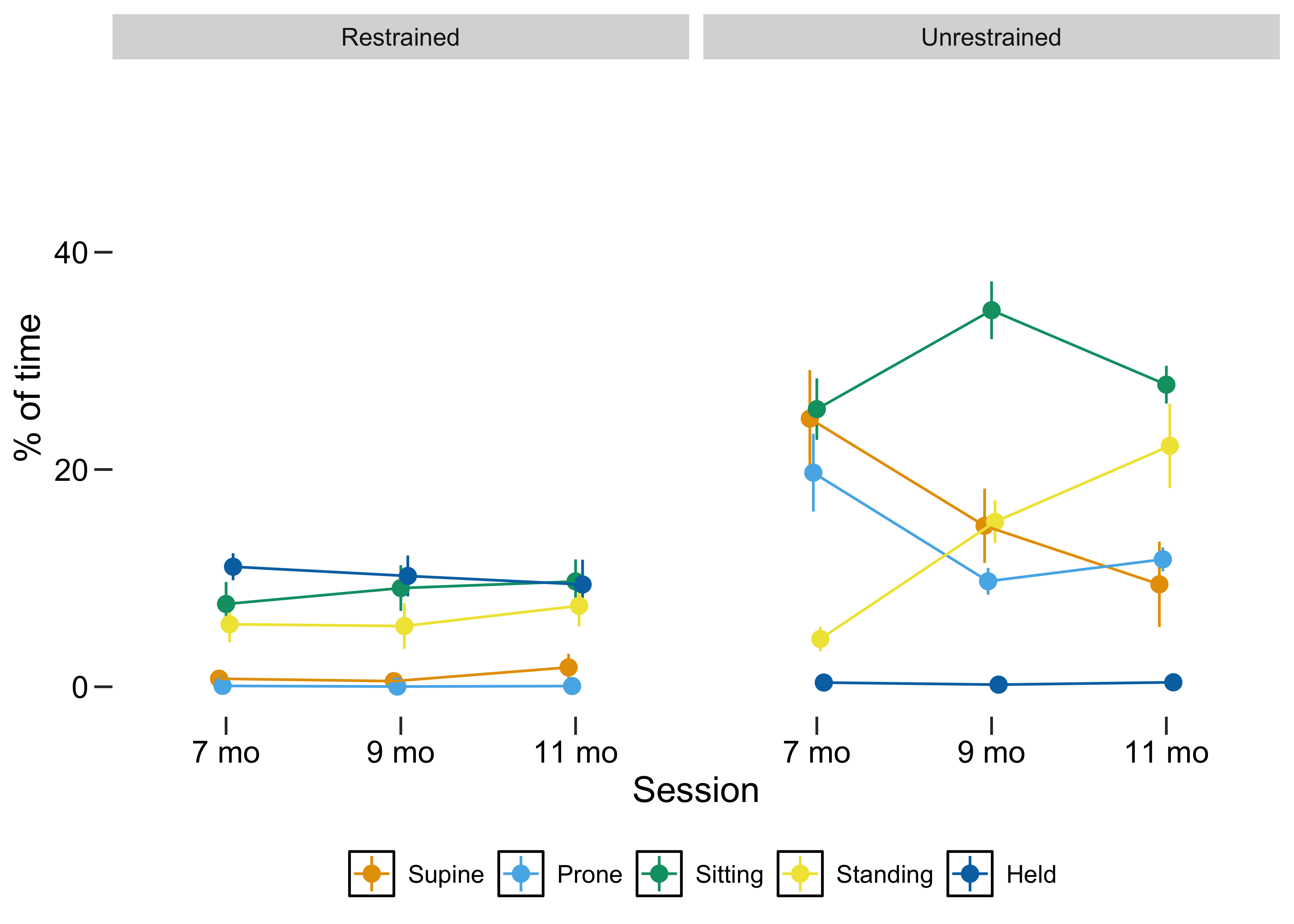
--- title: "Summaries" fig-dpi: 300 lightbox: auto execute: cache: false format: html: toc: true code-fold: true code-tools: true code-link: true knitr: opts_chunk: out.width: "100%" --- ```{r} #| echo: false #| warning: false #| error: false library (tidyverse)library (hms)library (rstatix)library (flextable)library (pins)<- c ("#F0E442" ,"#009E73" ,"#56B4E9" , "#E69F00" ,"#0072B2" ) %>% set_names (c ("Standing" , "Sitting" , "Prone" , "Supine" , "Held" ))<- c ("#CC79A7" ,"chartreuse4" ) %>% set_names (c ("Restrained" , "Unrestrained" ))theme_update (text = element_text (size = 12 ),axis.text.x = element_text (size = 12 , color = "black" ), axis.title.x = element_text (size = 14 ),axis.text.y = element_text (size = 12 , color = "black" ), axis.title.y = element_text (size = 14 ), panel.background = element_blank (),panel.border = element_blank (), panel.grid.major = element_blank (),panel.grid.minor = element_blank (), axis.line = element_blank (), axis.ticks.length= unit (.25 , "cm" ), legend.key = element_rect (fill = "white" )) <- board_folder ("/Volumes/padlab/study_sensorsinperson/data_processed/datasets/" )<- board %>% pin_meta ("imu_raw_samples" )<- board %>% pin_read ("imu_raw_samples" ) %>% filter (nap_period == 0 , exclude_period == 0 )``` `r round(now())` using pinned data version from: `r round(data_version$created)` ```{r} #| eval: false library (tidyverse)library (pins)library (nanoparquet)library (googledrive)# Load the board of pinned data sets (authenticated users only) <- board_gdrive (path = as_id ("1OZlphhu6vYm1A2Bm2-zD7a4luS5nGWgS" )) # To see available pinned data %>% pin_list ()# To read a specific data pin into memory <- board %>% pin_read ("imu_raw_samples" ) %>% filter (nap_period == 0 , exclude_period == 0 )``` ### Usable data ```{r} #| warning: false #| label: Usable-data #| tbl-cap: Usable data and total recording length in hours <- ds %>% count (id, session) %>% mutate (usable_hours = n/ 3600 )<- ds %>% group_by (id, session) %>% mutate (recording_hours = as.numeric (max (time) - min (time))) %>% slice_head (n = 1 ) %>% ungroup%>% left_join (recording_duration) %>% get_summary_stats (usable_hours, recording_hours, show = c ("mean" , "sd" ,"min" ,"max" )) %>% flextable () %>% autofit ()``` ```{r} #| warning: false #| label: Usable-data-histograms #| layout-ncol: 2 #| fig-cap: #| - "Usable hours after exclusions" #| - "Recording length in hours" %>% ggplot (aes (x = usable_hours)) + geom_histogram () + scale_x_binned (name = "Hours" , limits = c (2 ,14 ))%>% ggplot (aes (x = recording_hours)) + geom_histogram () + scale_x_binned (name = "Hours" , limits = c (2 ,14 ))``` ### Infant Position Frequency by Age (Overall) ```{r} #| warning: false #| label: position-table-age #| tbl-cap: Position summary statistics <- ds %>% group_by (id, session) %>% mutate (total_samples = n ()) %>% group_by (id, session, pos) %>% summarize (pos_n = n (), total_samples = mean (total_samples)) %>% ungroup<- ds_sum %>% complete (nesting (id, session), pos, fill = list (pos_n = 0 , total_samples = 1 ))$ pos_prop = ds_sum$ pos_n/ ds_sum$ total_samples* 100 $ session = as.numeric (ds_sum$ session)%>% group_by (pos, session) %>% get_summary_stats (pos_prop, show = c ("mean" , "sd" ,"min" ,"max" )) %>% select (- variable) %>% flextable () %>% autofit ()``` ```{r} #| warning: false #| label: "frequency-by-age-overall" #| layout-ncol: 2 #| fig-cap: #| - "Position means and SE" #| - "Position distribution" ggplot (ds_sum, aes (x = session, y = pos_prop, color = pos)) + stat_summary (position = position_dodge (.1 )) + stat_summary (geom = "line" , position = position_dodge (.1 )) + ylim (0 ,101 ) + ylab ("% of time" ) + xlab ("Session" ) + scale_x_continuous (breaks = 1 : 3 , labels = c ("7 mo" ,"9 mo" ,"11 mo" ), limits = c (0.5 ,3.5 )) + scale_color_manual (values = pal, name = "" ) + theme (legend.position = "bottom" )ggplot (ds_sum, aes (x = session, y = pos_prop, fill = pos)) + stat_summary (geom = "bar" , position = "stack" ) + ylim (0 ,101 ) + ylab ("% of time" ) + xlab ("Session" ) + scale_x_continuous (breaks = 1 : 3 , labels = c ("7 mo" ,"9 mo" ,"11 mo" ), limits = c (0.5 ,3.5 )) + scale_fill_manual (values = pal, name = "" ) + theme (legend.position = "bottom" )``` ### Infant Position Frequency by Age (Individual) ```{r} #| out-width: "90%" #| warning: false #| label: "frequency-by-age-individual" ggplot (ds_sum, aes (x = session, y = pos_prop, color = pos, group = id)) + facet_wrap (~ pos) + geom_point () + geom_line () + ylim (0 ,100 ) + ylab ("% of time" ) + xlab ("Session" ) + scale_x_continuous (breaks = 1 : 3 , labels = c ("7 mo" ,"9 mo" ,"11 mo" ), limits = c (0.5 ,3.5 )) + scale_color_manual (values = pal, name = "" ) + theme (legend.position = "none" )``` ### Infant Restraint Frequency by Age (Overall) ```{r} #| warning: false #| label: restraint-table-age #| tbl-cap: Restraint summary statistics <- ds %>% group_by (id, session) %>% mutate (total_samples = n ()) %>% group_by (id, session, restraint) %>% summarize (restraint_n = n (), total_samples = mean (total_samples)) %>% ungroup<- ds_sum_restraint %>% complete (nesting (id, session), restraint, fill = list (restraint_n = 0 , total_samples = 1 ))$ restraint_prop = ds_sum_restraint$ restraint_n/ ds_sum_restraint$ total_samples* 100 $ session = as.numeric (ds_sum_restraint$ session)%>% group_by (restraint, session) %>% get_summary_stats (restraint_prop, show = c ("mean" , "sd" ,"min" ,"max" )) %>% select (- variable) %>% flextable () %>% autofit ()``` ```{r} #| warning: false #| label: "restraint-by-age-overall" #| layout-ncol: 2 #| fig-cap: #| - "Restraint means and SE" #| - "Restraint distribution" ggplot (ds_sum_restraint, aes (x = session, y = restraint_prop, color = restraint)) + stat_summary (position = position_dodge (.1 )) + stat_summary (geom = "line" , position = position_dodge (.1 )) + ylim (0 ,101 ) + ylab ("% of time" ) + xlab ("Session" ) + scale_x_continuous (breaks = 1 : 3 , labels = c ("7 mo" ,"9 mo" ,"11 mo" ), limits = c (0.5 ,3.5 )) + scale_color_manual (values = restraint_pal, name = "" ) + theme (legend.position = "bottom" )ggplot (ds_sum_restraint, aes (x = session, y = restraint_prop, fill = restraint)) + stat_summary (geom = "bar" , position = "stack" ) + ylim (0 ,101 ) + ylab ("% of time" ) + xlab ("Session" ) + scale_x_continuous (breaks = 1 : 3 , labels = c ("7 mo" ,"9 mo" ,"11 mo" ), limits = c (0.5 ,3.5 )) + scale_fill_manual (values = restraint_pal, name = "" ) + theme (legend.position = "bottom" )``` ### Infant Restraint Frequency by Age (Individual) ```{r} #| out-width: "90%" #| warning: false #| label: "restraint-by-age-individual" ggplot (ds_sum_restraint, aes (x = session, y = restraint_prop, color = restraint, group = id)) + facet_wrap (~ restraint) + geom_point () + geom_line () + ylim (0 ,100 ) + ylab ("% of time" ) + xlab ("Session" ) + scale_x_continuous (breaks = 1 : 3 , labels = c ("7 mo" ,"9 mo" ,"11 mo" ), limits = c (0.5 ,3.5 )) + scale_color_manual (values = restraint_pal, name = "" ) + theme (legend.position = "none" )``` ### Posture by restraint ```{r} #| out-width: "90%" #| warning: false #| label: "posture-by-restraint" <- ds %>% group_by (id, session) %>% mutate (total_samples = n ()) %>% group_by (id, session, pos, restraint) %>% summarize (posrest_n = n (), total_samples = mean (total_samples)) %>% ungroup<- ds_sum_posrest %>% complete (nesting (id, session), restraint, pos, fill = list (posrest_n = 0 , total_samples = 1 ))$ prop = ds_sum_posrest$ posrest_n/ ds_sum_posrest$ total_samples* 100 $ session = as.numeric (ds_sum_posrest$ session)ggplot (ds_sum_posrest, aes (x = session, y = prop, color = pos)) + stat_summary (position = position_dodge (.1 )) + stat_summary (geom = "line" , position = position_dodge (.1 )) + facet_wrap (~ restraint) + ylab ("% of time" ) + xlab ("Session" ) + scale_x_continuous (breaks = 1 : 3 , labels = c ("7 mo" ,"9 mo" ,"11 mo" ), limits = c (0.5 ,3.5 )) + coord_cartesian (ylim = c (0 ,55 )) + scale_color_manual (values = pal, name = "" ) + theme (legend.position = "bottom" )```